The Supply Side of Chiropractic Services: Do Doctors Work More for Less, or Less for Less?*

The analysis that follows is not necessarily for everyone. Although anyone can and is invited to work through it, those readers who have been exposed to even a little bit of formal economics (perhaps long enough ago to seem a previous lifetime) will have an easier time of it. I will not be insulted by anyone who skips right to my conclusions near the end, the part where I explain why, thanks to managed care, so many chiropractors wind up working more for less (like my office-mate), and others (like me) wind up working less for less.

Optimizing the Leisure-Income Tradeoff Subject to a Budgetary Constraint

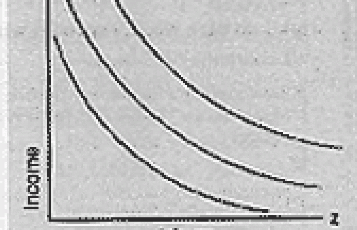
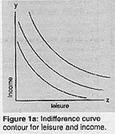
Income-Leisure Indifference Curves

Since a doctor has to give up leisure to earn income (or commodities), we can construct a group of indifference curves that show the individual doctor's subjective tradeoff between the two, at various levels of satisfaction. Figure 1a shows such a family of indifference curves. At any point on a curve, the doctor derives equal utility (i.e., satisfaction) from the associated combination of leisure and income. As the doctor moves along the curve, he substitutes leisure for income, but remains equally satisfied with the outcome. The doctor prefers more northeasterly indifference curves that permit more leisure and income, say, following a rise in his income, but is glad not to be on more southwesterly curves, where a tax increase would put him.

Income-Leisure Feasibility Line

Suppose the doctor has a total of T hours available for either work or leisure. He divides this time between h hours of work and z hours of leisure, receives a wage rate w, and earns an income y. Under these assumptions, the following equations may be written:

By eliminating the variable h from this pair of simultaneous equations, we derive y=-w(z-T), the equation of the line in figure 1b. This income-leisure feasibility line shows the objective exchange rate at which units of income may be "spent" on leisure, what amounts to a budgetary constraint. In other words, the doctor is able to convert income to leisure by working less, and leisure to income by working more, at a fixed rate as given by the his time to work and earns an income of wT. At the x intercept, the doctor spends all his time on leisure and earns no income. Since the slope of the line is -w, the wage rate is also the price of leisure. Every hour the doctor does not work is equivalent to a purchase of leisure, at the price of -w/hour.

Figure 1b: Income-leisure budgetary constraint line.

Utility (satisfaction) Optimization

It can be shown that if the doctor chooses to maximize his utility, subject to the constraint of the income-leisure line, he will choose to earn an income Y* and enjoy z* hours of leisure, as seen in Figure 1c. This is the point where the highest attainable subjective preferences curve is tangent to the income-leisure line. No other point on his indifference curve can be attained at wage rate w (they would be too costly), and no other point on the income-leisure line would provide as much utility.

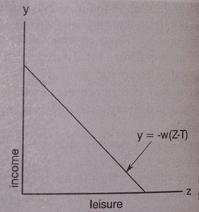
Figure 1c: Optimizing utility subject to budgetary constraint.

Effects of Diminishing the Wage Rate

Let us now see what happens were w, the wage rate, to decrease to w*, perhaps due to the effects of managed care. The wage rate need not be an actual hourly wage. It can be understood as an imputed wage paid by a self-employed doctor to himself. Graphically, this would make the income-leisure line less steep, rotating it counter-clockwise around the x intercept, as seen in Figure 2a, where income y=-w*(z-T). The doctor must fall to a more southwesterly, lower indifference curve, but there are three ways this can happen, each of which is shown in Figures 2b-d. As before, the optimal solution for the doctor is where a subjective preferences curve is tangent to the (new) income-leisure line, at (z', y') but we cannot predict a priori to which of the three curves he will fall. That is a question of the individual doctor's subjective preferences.

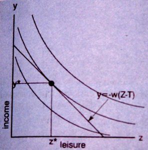
Figure 2a: Income-leisure line shifts due to decreased wage rate.]

Let us examine the three possible outcomes of a wage cut, explain the results, and then provide a character sketch for each of the three types of doctor.

In Figure 2b, the doctor works more, earns more income, and consumes less leisure.

In Figure 2c, the doctor works more, earns less income, and consumes less leisure.

In Figure 2d, the doctor works less, earns less income, and consumes more leisure.

How and why these results come about can be understood as the net effect of two possible doctor responses to lower wage rates, that are opposite in direction:

Substitution effect: Since doctors "purchase" their leisure time by forgoing the fruits of their labor, the wage rate is effectively the price of leisure. As the wage rate decreases, they shift their time away from income generation toward leisure, as leisure becomes relatively cheaper.

Income effect: Lower hourly wage rates result in less income, and thus decreased demand for all (normal) goods, including leisure. Thus, decreased income decreases the demand for leisure.

Summarizing: When rate rates decline, the substitution effect increases the doctors's demand for leisure (decreases his work effort), whereas the income effect decreases his demand for leisure (increases his work effort). In Figures 2b and 2c, the income effect dominates, whereas in Figure 2d the substitution effect dominates.

Figure 2b: At new optimization point, income effect dominates, income rises, leisure drops.

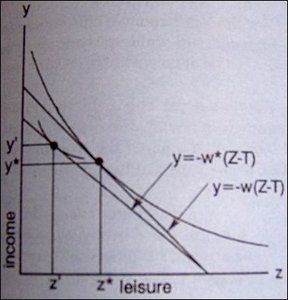
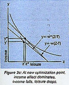
Let us paint a character profile to better understand the outcome. When wages fall, some doctors will attempt so hard to preserve their income and standard of living that they will respond by working harder (Figures 2b-c), so much so that they might actually wind up increasing their income in spite of the decline in wage rates (Figure 2b). On the other hand, when wages fall, some doctors will so little appreciate the rewards of working at that lower wage, that they decide to enjoy more leisure instead, accepting the consequence of a reduced level of consumption for everything but leisure (Figure 2d). This doctor withdraws labor, only too happy to sacrifice income, because it is literally not worth the trouble at the lower wage rate.

The Backward Bending Supply Curve for Labor

Supply curves show the amount of a commodity that a producer is willing to supply in exchange for various prices. In most markets, the supply curve continuously increases to the right, because suppliers are more than happy to offer more goods at higher prices, as seen in Figure 3a. Labor markets, on the other hand, may not conform to this usual model. Some economists believe that in labor markets, the supply curve is backward bending, as seen in figure 3b.

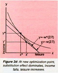
Figure 3a: Typical supply curve, showing increased offering at increasing prices.

Figure 3b: Backward bending supply curve, with divergent responses to wage rate cuts.

As wage rates increase, there comes a point where workers actually withdraw labor from the market. We have already seen how this could happen, since it would merely be the flip side of the effect noted in figures 2b-c, where doctors increased their effort when wage rates fell. There are no data to my knowledge to confirm that the supply curve for chiropractic labor is backward bending in the aggregate, but there is little doubt that the supply curve for some doctors is backward bending. Perhaps at high income levels, doctors earn so much that their leisure becomes relatively more valuable than income.

Economic studies have shown that workers who earn a high wage rate are more likely to work harder when wage rates decrease (work less when wage rates increase), whereas those paid a lower rate are more likely to withdraw their labor from the market when wage rates decline (supply more labor when wage rates increase). Those better paid workers in Figure 2b-c are the ones who contribute to the backward bending portion of the supply curve in Figure 3b, sections a and b of the curve. Indeed, the income effect is so pronounced in region a, as the label suggests, that when a small dip in wage rates calls forth a large increase in work effort, their income actually increases. The less well-paid worker in Figure 2d accounts for region c of the curve in Figure 3b, the more typical scenario: lower prices call forth a smaller supply of the commodity or service in question. There, the substitution effect dominates over the income effect, as the label on the curve indicates.

Although it remains to be seen whether empirical studies will verify that better paid chiropractors work harder when managed care bites, while lower paid chiropractors respond by cutting back, we are not entirely without evidence. A tax lawyer, studying his wealthy friends, found that increased taxes caused them to work harder, presumably to maintain their previous standard of living. On the other hand, it would be premature to suggest that in the aggregate, decreasing doctor incomes would just make them work harder (ouch), as some social engineers have suggested in support of redistributionist schemes and socialized medicine.

This analysis of how doctor labor supplies respond to wage rate changes may explain or even predict changes in the market for chiropractic labor inputs at a time when an increasing level of managed care and other negotiated price cuts may very well be reducing chiropractor's hourly wage rates (employee or imputed). Economic theory and even some data predict that the representative chiropractor at the high end will wind up working more for less, while at the low end, less for less.

*This column is based on an article in review with Topics in Physician-Firm." Robert Cooperstein, MA, DC
Administrative Research Coordinator
Chairman of the Technique Department
Palmer College of Chiropractic West
San Jose, California
drrcoop-aol.com